Introduction
We will demonstrate how to use ctSVG to identify cell-type-specific SVGs with cell type annotations from Xenium data. The Xenium dataset of a human lung cancer sample was downloaded from the 10x website.
Load package
library(ctSVG)
mydir <- "~/Desktop/Research/ctSVG/xenium_human_lungcancer"
list.files(mydir)
#> [1] "coord.rds" "expr.rds"  "sc.rds"
expr <- readRDS(file.path(mydir, "expr.rds"))
coord <- readRDS(file.path(mydir, "coord.rds"))
sc <- readRDS(file.path(mydir, "sc.rds"))
str(expr)
#> Formal class 'dgCMatrix' [package "Matrix"] with 6 slots
#>   ..@ i       : int [1:4838175] 4 76 81 97 160 203 249 283 287 293 ...
#>   ..@ p       : int [1:151678] 0 15 53 71 104 166 198 232 274 305 ...
#>   ..@ Dim     : int [1:2] 377 151677
#>   ..@ Dimnames:List of 2
#>   .. ..$ : chr [1:377] "ABCC11" "ACE2" "ACKR1" "ACTA2" ...
#>   .. ..$ : chr [1:151677] "aaaaficg-1" "aaabbaka-1" "aaabbjoo-1" "aaablchg-1" ...
#>   ..@ x       : num [1:4838175] 6.27 6.27 6.27 6.27 6.27 ...
#>   ..@ factors : list()
str(coord)
#>  num [1:151677, 1:2] 202 179 186 200 197 ...
#>  - attr(*, "dimnames")=List of 2
#>   ..$ : chr [1:151677] "aaaaficg-1" "aaabbaka-1" "aaabbjoo-1" "aaablchg-1" ...
#>   ..$ : chr [1:2] "row" "col"
str(sc)
#>  Factor w/ 14 levels "0","1","2","3",..: 10 3 2 2 3 1 2 11 2 2 ...
#>  - attr(*, "names")= chr [1:151677] "aaaaficg-1" "aaabbaka-1" "aaabbjoo-1" "aaablchg-1" ...
sc <- sc[sc %in% levels(sc)[1:3]]
sc <- droplevels(sc)
Identify spatially variable genes within each cell cluster
suppressMessages(suppressWarnings(
  clutestRes <- ctsvg_test(expr = expr, coord = coord, sc = sc)
))
head(clutestRes)
#>         cluster  gene fdr    logpval pval    fstat knotnum
#> 0.MYC         0   MYC   0 -4311.2679    0 695.6332       0
#> 0.BASP1       0 BASP1   0 -1441.4703    0 209.6989       0
#> 0.MET         0   MET   0 -1366.8257    0 198.4745       0
#> 0.PCSK2       0 PCSK2   0 -1131.1431    0 163.4559       0
#> 0.TCIM        0  TCIM   0  -998.8474    0 144.0727       0
#> 0.TNC         0   TNC   0  -780.9037    0 112.5533       0
Fit spatial gene expression patterns within each cell cluster
clufitRes <- ctsvg_fit(expr = expr, coord = coord, sc = sc)Visualize spatial patterns of a single gene
plotGene(expr = expr, clufitRes = clufitRes, coord = coord, sc = sc,
         gene = clutestRes$gene[1], cellclu = "0", background = TRUE)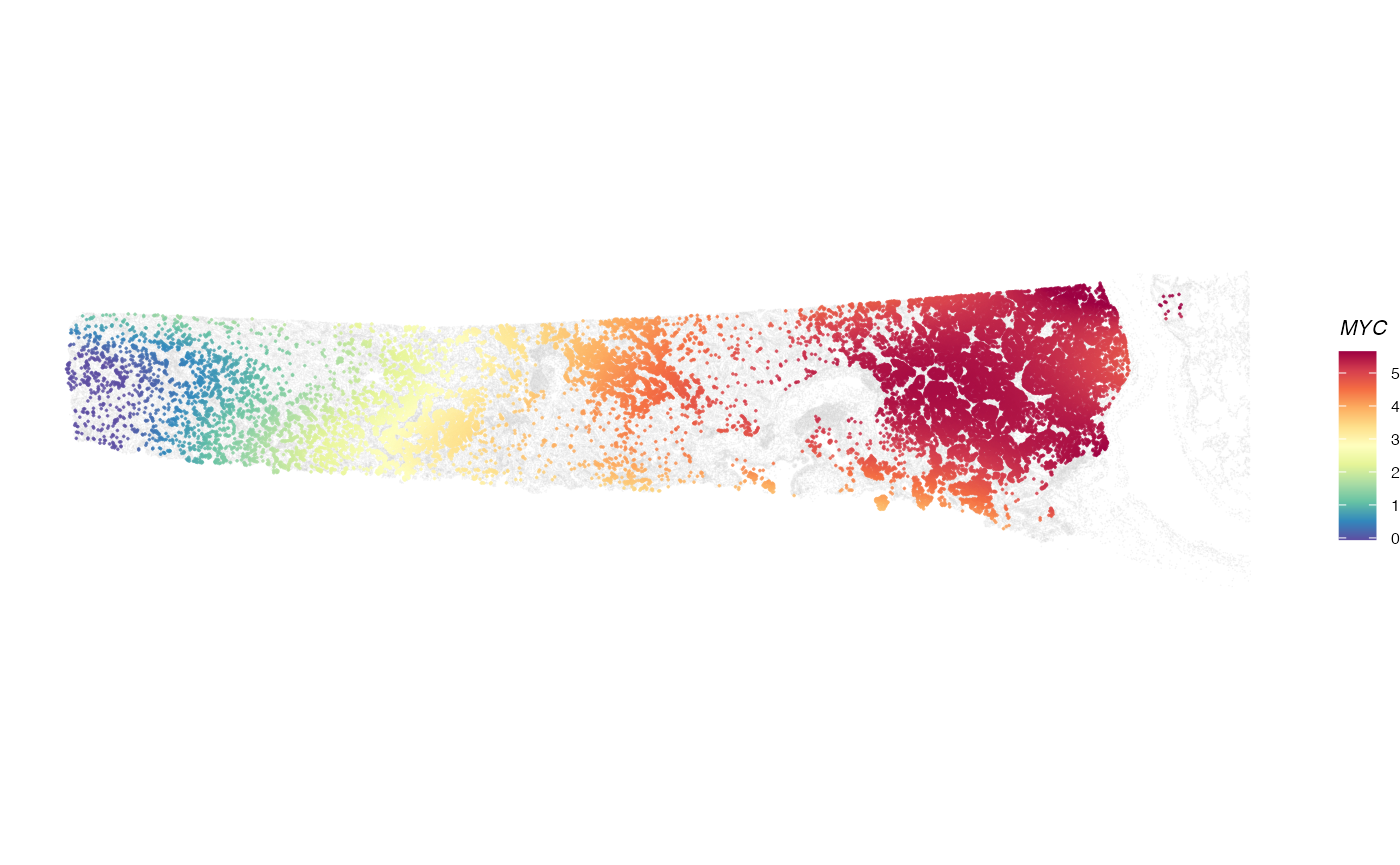
Identify gene modules within each cell cluster
moduleRes <- ctsvg_module(clutestRes = clutestRes, clufitRes = clufitRes, sc = sc)Visualize spatial patterns of metagenes within a cell cluster
plotMetagene(clufitRes = clufitRes, coord = coord, sc = sc,
             moduleRes = moduleRes, cellclu = "0", background = TRUE)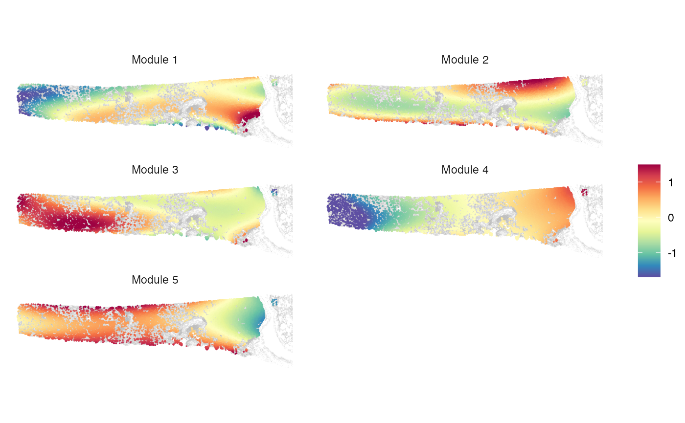
Session Info
sessionInfo()
#> R version 4.4.1 (2024-06-14)
#> Platform: aarch64-apple-darwin20
#> Running under: macOS 15.6.1
#>
#> Matrix products: default
#> BLAS:   /Library/Frameworks/R.framework/Versions/4.4-arm64/Resources/lib/libRblas.0.dylib
#> LAPACK: /Library/Frameworks/R.framework/Versions/4.4-arm64/Resources/lib/libRlapack.dylib;  LAPACK version 3.12.0
#>
#> locale:
#> [1] en_US.UTF-8/en_US.UTF-8/en_US.UTF-8/C/en_US.UTF-8/en_US.UTF-8
#>
#> time zone: America/New_York
#> tzcode source: internal
#>
#> attached base packages:
#> [1] stats     graphics  grDevices utils     datasets  methods   base
#>
#> other attached packages:
#> [1] ctSVG_1.0
#>
#> loaded via a namespace (and not attached):
#>   [1] RColorBrewer_1.1-3     rstudioapi_0.16.0      jsonlite_1.8.8
#>   [4] magrittr_2.0.3         spatstat.utils_3.1-0   farver_2.1.2
#>   [7] rmarkdown_2.28         fs_1.6.4               ragg_1.3.2
#>  [10] vctrs_0.6.5            ROCR_1.0-11            spatstat.explore_3.3-2
#>  [13] htmltools_0.5.8.1      findPC_1.0             sass_0.4.9
#>  [16] sctransform_0.4.1      parallelly_1.38.0      KernSmooth_2.23-24
#>  [19] bslib_0.8.0            htmlwidgets_1.6.4      desc_1.4.3
#>  [22] ica_1.0-3              plyr_1.8.9             plotly_4.10.4
#>  [25] zoo_1.8-12             cachem_1.1.0           igraph_2.0.3
#>  [28] mime_0.12              lifecycle_1.0.4        pkgconfig_2.0.3
#>  [31] Matrix_1.7-0           R6_2.5.1               fastmap_1.2.0
#>  [34] fitdistrplus_1.2-1     future_1.34.0          shiny_1.9.1
#>  [37] digest_0.6.37          colorspace_2.1-1       patchwork_1.3.0
#>  [40] Seurat_5.1.0           tensor_1.5             RSpectra_0.16-2
#>  [43] irlba_2.3.5.1          textshaping_0.4.0      labeling_0.4.3
#>  [46] progressr_0.14.0       fansi_1.0.6            spatstat.sparse_3.1-0
#>  [49] httr_1.4.7             polyclip_1.10-7        abind_1.4-8
#>  [52] compiler_4.4.1         proxy_0.4-27           withr_3.0.1
#>  [55] DBI_1.2.3              fastDummies_1.7.4      highr_0.11
#>  [58] MASS_7.3-60.2          classInt_0.4-10        units_0.8-5
#>  [61] tools_4.4.1            lmtest_0.9-40          httpuv_1.6.15
#>  [64] future.apply_1.11.2    goftest_1.2-3          glue_1.7.0
#>  [67] nlme_3.1-164           promises_1.3.0         grid_4.4.1
#>  [70] sf_1.0-18              Rtsne_0.17             cluster_2.1.6
#>  [73] reshape2_1.4.4         generics_0.1.3         gtable_0.3.5
#>  [76] spatstat.data_3.1-2    class_7.3-22           tidyr_1.3.1
#>  [79] data.table_1.16.2      sp_2.1-4               utf8_1.2.4
#>  [82] spatstat.geom_3.3-3    RcppAnnoy_0.0.22       ggrepel_0.9.6
#>  [85] RANN_2.6.2             pillar_1.9.0           stringr_1.5.1
#>  [88] spam_2.11-0            RcppHNSW_0.6.0         later_1.3.2
#>  [91] splines_4.4.1          dplyr_1.1.4            lattice_0.22-6
#>  [94] survival_3.6-4         deldir_2.0-4           tidyselect_1.2.1
#>  [97] miniUI_0.1.1.1         pbapply_1.7-2          knitr_1.48
#> [100] gridExtra_2.3          scattermore_1.2        xfun_0.47
#> [103] matrixStats_1.3.0      stringi_1.8.4          lazyeval_0.2.2
#> [106] yaml_2.3.10            evaluate_0.24.0        codetools_0.2-20
#> [109] tibble_3.2.1           cli_3.6.3              uwot_0.2.2
#> [112] xtable_1.8-4           reticulate_1.39.0      systemfonts_1.1.0
#> [115] munsell_0.5.1          jquerylib_0.1.4        Rcpp_1.0.13
#> [118] globals_0.16.3         spatstat.random_3.3-2  png_0.1-8
#> [121] spatstat.univar_3.0-1  parallel_4.4.1         pkgdown_2.1.0
#> [124] ggplot2_3.5.1          dotCall64_1.2          listenv_0.9.1
#> [127] viridisLite_0.4.2      e1071_1.7-16           scales_1.3.0
#> [130] ggridges_0.5.6         SeuratObject_5.0.2     leiden_0.4.3.1
#> [133] purrr_1.0.2            rlang_1.1.4            cowplot_1.1.3